When you want to start creating a map, often the first thing you need is the actual country shapes. In mapping terms these edges are called administrative boundaries. There are a few different free and online sources for this data. Two popular datasets are called Global Administrative Areas (GADM) and Natural Earth. In this article we will compare both options, and visualize the data using Python.

As a proof of concept I will use the administrative boundaries of the Netherlands. This country is interesting, first of all, because it is where I’m from, but also because it has a large interior lake, and some Islands in the Caribbean. So it is interesting to see how this is handled in the data.

GADM

GADM is an open dataset, that can be found here, and is consolidated from different sources. I have downloaded the data for the entire world, in the GeoPackage file format.

Reading in the data

In this article I have explained how to set up your Python environment for creating maps using GeoPandas. The simplest way to open the GADM GeoPackage is with this code:

import geopandas as gpd

boundaries = gpd.read_file('gadm_410.gpkg')

However, since this file is almost 2.7 GB, reading it into a GeoDataFrame is very slow, and on my machine takes 508 seconds. Way too much for just creating a simple map.

As explained here, behind the screens the Fiona package is used to link to GDAL for reading the file. There is an alternative package which is called pyogrio, and which promises to be faster. But we have to explicitly tell GeoPandas to use this newer driver.

boundaries = gpd.read_file('gadm_410.gpkg', engine='pyogrio')

With this approach, the runtime drops to 34 seconds, a huge improvement.

Since the data is actually fist read in using GDAL C/C++ code, its content needs to be transfered to the Python memory. There is a more efficient way to do this, using Arrow, a standard in-memory data format. If both GDAL and Python were to use this, handing over the data is as simple as passing a pointer, without the need to copy the data itself. To do this, install the arrow drivers using conda install -c conda-forge libgdal-arrow-parquet pyarrow, and then add the following option:

boundaries = gpd.read_file('gadm_410.gpkg', engine='pyogrio', use_arrow=True)

Now we are down to 11 seconds, which is almost 50 times faster than the first code, just by adding two small options.

Analyzing the data

At this point the data is still a black box. A convenient way to browse through the data if you are developing with Visual Studio Code is by opening the variable in the Data Wrangler extension, and to be fair, it’s also very convenient to do this in QGIS. Alternatively you can use Python commands to understand the structure of the dataset. Like for example:

print(boundaries.columns)
print(boundaries.query("NAME_0=='Netherlands'")['NAME_1'].unique())
print(boundaries.query("NAME_0=='Netherlands'")['TYPE_1'].unique())

This returns the column names, as well as selected values for some columns:

Index(['UID', 'GID_0', 'NAME_0', 'VARNAME_0', 'GID_1', 'NAME_1', 'VARNAME_1',
       'NL_NAME_1', 'ISO_1', 'HASC_1', 'CC_1', 'TYPE_1', 'ENGTYPE_1',
       'VALIDFR_1', 'GID_2', 'NAME_2', 'VARNAME_2', 'NL_NAME_2', 'HASC_2',
       'CC_2', 'TYPE_2', 'ENGTYPE_2', 'VALIDFR_2', 'GID_3', 'NAME_3',
       'VARNAME_3', 'NL_NAME_3', 'HASC_3', 'CC_3', 'TYPE_3', 'ENGTYPE_3',
       'VALIDFR_3', 'GID_4', 'NAME_4', 'VARNAME_4', 'CC_4', 'TYPE_4',
       'ENGTYPE_4', 'VALIDFR_4', 'GID_5', 'NAME_5', 'CC_5', 'TYPE_5',
       'ENGTYPE_5', 'GOVERNEDBY', 'SOVEREIGN', 'DISPUTEDBY', 'REGION',
       'VARREGION', 'COUNTRY', 'CONTINENT', 'SUBCONT', 'geometry'],
      dtype='object')

['Drenthe' 'Flevoland' 'Fryslân' 'Gelderland' 'Groningen' 'IJsselmeer'
 'Limburg' 'Noord-Brabant' 'Noord-Holland' 'Overijssel' 'Utrecht'
 'Zeeland' 'Zeeuwse meren' 'Zuid-Holland' 'Zuid Hollandse Meren']

['Provincie' 'Water body']

In summary, it turns out that the GADM dataset contains a single row for each smallest administrative boundary, like a municipality. There are no separate rows for higher level entities such as provinces or entire countries.

Visualizing the data

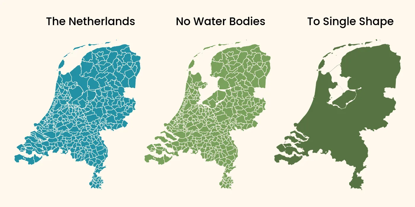
With this information, we know that we need to consolidate all municipality boundaries into a single shape, and subtract the water bodies which are also present in the GADM data. This we can do with GeoPandas as follows:

the_netherlands = boundaries.query("NAME_0 == 'Netherlands'")
no_water_bodies = the_netherlands.query("TYPE_1 != 'Water body'")
to_single_shape = no_water_bodies.dissolve(by='NAME_0')

to_single_shape.plot()

These three different variables are visualized below.

Faster execution with GDAL

Reading and plotting the map of the Netherlands with the previous code takes a total of 19 seconds. However, as a rule of thumb it is faster to push as much of the code to the C/C++ GDAL layer, since it executes way faster than Python code.

GDAL, through GeoPandas with the pyogrio package can query data with SQL and SpatiaLite commands for geospatial operations. The ST_Union function in the query below will already join the different subregions into a single shape, resulting in the same final output as the GeoPandas commands used before.

country = gpd.read_file('gadm_410.gpkg', 
    engine='pyogrio', 
    use_arrow=True, 
    sql='''
            SELECT ST_Union(geom)  
            FROM gadm_410
            WHERE 
                ENGTYPE_1 != "Water body" 
                AND NAME_0 = "Netherlands"
        ''')

country.plot()

The drawback is that you need some understanding of basic SQL for this approach, but the benefit is that the total execution time is again reduced more than 6 times, to less than 3 seconds.

Natural Earth

Where GADM is a dataset that contains just the administrative boundaries, Natural Earth is a much richer dataset, with open data for many different map layers, to be able to create complete maps from scratch, while still remaining relatively small in size. It does this by excluding detail, meaning the dataset is more suited for creating country or region maps.

Reading the data

Different data formats are offered, but the default download comes ESRI shapefiles. With the Natural Earth data, we need to use two files. One for the country shapes, and one for the lakes. Especially in case of the Netherlands, where the IJsselmeer is a defining feature. For the country shapes, multiple files are provided, but we select the one for so-called map units, since otherwise the Dutch Caribbean would be included as well.

One drawback of the dataset, is that the lakes have no attribute linking it to the countries. Therefore we either need to select manually which lake we want to subtract, or to be more generic, subtract all lakes, like so:

netherlands = gpd.read_file('ne_10m_admin_0_map_units.shp', 
                            engine='pyogrio', 
                            use_arrow=True,
                            where="NAME = 'Netherlands'")

lakes = gpd.read_file('ne_10m_lakes.shp', engine='pyogrio', use_arrow=True)

result = netherlands.overlay(lakes, how='difference')

result.plot()

Visualizing the data

The Natural Earth data comes in three different scales, 1:10 million, 1:50 million and 1:110 million. These are provided in different subfolders with clear file naming. Below you can see what these three different levels of detail look like.

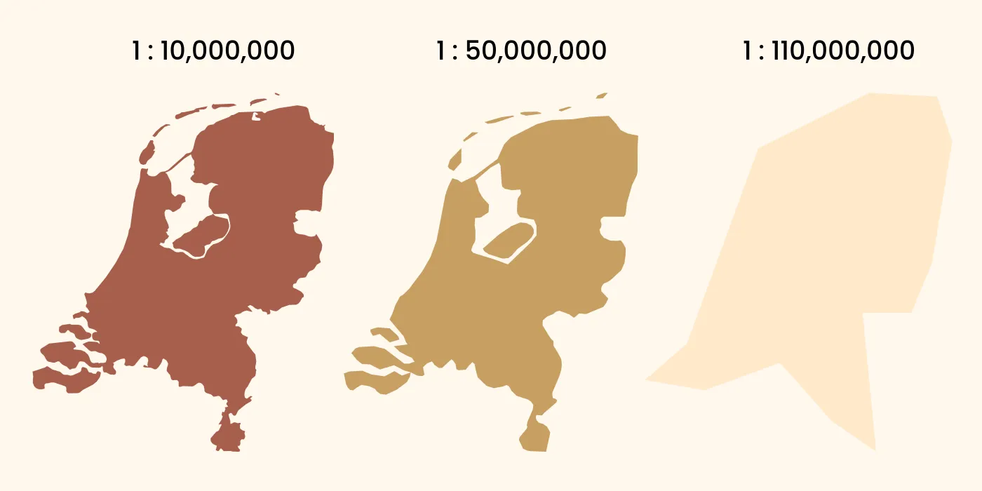
Obviously this visualization is not to scale, but it shows the differences in the three different datasets. It also makes clear that the GADM data simply contains the geometries at the highest fidelity possible, and that this is not always desirable. For me the Natural Earth data looks most visually pleasing at this scale, and simplification algorithms would be needed to achieve the same with the GADM data. But that is a topic for another day.